# Installing resquin
install.packages("resquin")
# Loading resquin into the R session
library(resquin)Reproduce information
Resquin
Assessing Response Quality and Careless Responding in Multi-Item Scales
Last update on May 19, 2025.
At a glance
What do we need to be aware of when analyzing responses of multi-item scales? Which response quality issues can affect data from multi-item scales? This tool gives an overview on the assessment of response quality in multi-item scales and guides you through the quality analysis with replicable R-code. Specifically, you will learn:
how to calculate and interpret different indicators of response distribution regarding potential data quality issues,
how to calculate and interpret indicators of different response styles which can reflect poor response behavior,
the caveats of certain response quality indicators and their suitability for different question types and response scales,
what to do if you detect poor quality responses.
Table of Content
Introduction
Psychological constructs, political or social attitudes as well as behavioral patterns are often measured by using multi-item scales in questionnaires. Multi-item scales comprise several items, questions, or statements that assess different aspects of the same underlying construct, i.e., gender-role attitudes or attitudes toward foreigners. Main concerns of multi-item scales usually revolve around the validity of the measurement instrument itself, i.e., do the several questions/items reflect the underlying construct or in other words: Does the scale really measure what it intends to measure? Established scales usually underwent a series of analyses and revisions to assess and ensure the validity and reliability of the measurement instrument. Nevertheless, collected data from these scales can still suffer from bias resulting from poor response behavior. Before analyzing data from these scales and drawing conclusions regarding a substantive research question, the quality of survey responses to these scales should be examined to avoid bias and ensure the validity of your results. In this tutorial, we will focus on the relationship between the concepts of political/institutional trust and environmental attitudes which both are measured by multi-item scales and assess the quality of given responses to these scales.
Set-up
Data and Measurement Instruments
For this tutorial, we use data from the GESIS Panel. The GESIS Panel is a German probability-based mixed-mode panel study which surveys respondents every three months on a variety of topics, such as political and social attitudes. We specifically use data from the 2nd and 3rd wave in 2014 from a sub-sample of the GESIS Panel (n=1,222). The data includes multi-item measurements of political trust and environmental attitudes.
Note
This sub-sample of the GESIS Panel (2017) is publicly accessible as the GESIS Panel Campus File. It contains a random 25% sample of the GESIS panel members surveyed in 2014 and comprises only a limited selection of variables from the originial GESIS Panel scientific use file.
Political trust is measured with a 10-item scale and a 7-point Likert response scale:
Trust in Institutions: Trust in various political institutions
How much do you personally trust the following public institutions or groups?
| Items | Institution |
|---|---|
| bbzc078a | Trust in Bundestag |
| bbzc079a | Trust in federal government |
| bbzc080a | Trust in political parties |
| bbzc081a | Trust in judicial authorities |
| bbzc082a | Trust in police |
| bbzc083a | Trust in politicians |
| bbzc084a | Trust in media |
| bbzc085a | Trust in European Union |
| bbzc086a | Trust in United Nations |
| bbzc087a | Trust in Federal Constitutional Court |
Response Scale: 1 = Don’t trust at all - 7 = Entirely trust
Environmental attitudes are measured with the established NEP (New Ecological Paradigm) scale by Dunlap et al. (2002) comprising 15 items on different aspects of environmental or climate attitudes. The multi-item scale uses a 5-point Likert response scale.
NEP scale: Environmental attitudes
To what extent do you agree or disagree with the following statements?
Items:
- bczd005a: NEP-scale: Approaching maximum number of humans
- bczd006a: NEP-scale: The right to adapt environment to the needs
- bczd007a: NEP-scale: Consequences of human intervention
- bczd008a: NEP-scale: Human ingenuity
- bczd009a: NEP-scale: Abuse of the environment by humans
- bczd010a: NEP-scale: Sufficient natural resources
- bczd011a: NEP-scale: Equal rights for plants and animals
- bczd012a: NEP-scale: Balance of nature stable enough
- bczd013a: NEP-scale: Humans are subjected to natural laws
- bczd014a: NEP-scale: Environmental crisis greatly exaggerated
- bczd015a: NEP-scale: Earth is like spaceship
- bczd016a: NEP-scale: Humans were assigned to rule over nature
- bczd017a: NEP-scale: Balance of nature is very sensitive
- bczd018a: NEP-scale: Control nature
- bczd019a: NEP-scale: Environmental disaster
Response Scale: 1 = Fully agree; 2 = Agree; 3 = Neither nor; 4 = Don’t agree; 5 = Fully disagree
Assessing Response Quality and Response Quality Indicators
To ensure unbiased conclusions regarding a substantial relationship between two construct, we advise to initially investigate the quality of given responses to the respective measurement instruments. There are several indicators which can help identify low-quality responses and assess the response quality in multi-item scales.
In this tutorial, we will specifically look at several indicators of response distribution, such as:
- The proportion of missing responses across multiple items per respondent (
prop_na) - The mean over multiple items per respondent (
ii_mean) - The median over multiple items per respondent (
ii_median) - The standard deviation across multiple items per respondent (
ii_sd) - The Mahalanobis distance: The Mahalanobis distance captures how different each respondent’s pattern of answers is from the ‘typical’ response pattern of all respondents. A higher score indicates that the respondent’s answers are more unusual or inconsistent compared to the other respondents.
Apart from peculiarities in the response distribution of our multi-item scales, we will further consider indicators of different response biases, namely:
MRS: Middle response style
Tendency to select the neutral/middle option on a scale: The indicator captures the sum of mid-point responses across the items of the scale and is only valid if the scale has a numeric midpoint.
ARS: Acquiescence response style
Tendency to agree with statements irrespective of actual views. The indicator captures the sum of responses above the scale mid-point across the items of a scale and is only valid for scales with an agree-disagree format.
ERS: Extreme response style
Tendency to select the lower or upper endpoint of a scale. The indicator captures the sum of scale endpoint responses across the items of a scale.
To calculate these indicators for the assessment of response quality of our multi-item scales, we will use the Resquin package in R (Roth et al. 2024). The resquin package comprises different functions to calculate response quality indicators for multi-item scales. The quality indicators are calculated per respondent. Specifically, we will use the two functions resp_distributions (indicators of response distribution) and resp_styles(response style indicators), designed to assess response quality based on response distribution and on identifying certain response biases.
Getting started
To use resquin, we first need to install the package from the repository of CRAN, the Comprehensive R Archive Network. For installation, we can use the following commands:
Alongside resquin itself, we will use other packages for setup, data preparation and analysis in this tutorial. To install and load these packages from CRAN simultaneously, we will use the pacman package:
# Installing pacman and loading pacman into the R session
install.packages("pacman")
library(pacman)

# Install and load other CRAN packages using pacman
pacman::p_load(devtools, pak, dplyr,ggplot2,tidyr,patchwork, knitr, kableExtra)
After installation, we can import the survey data we want to analyze regarding its response quality. For both resp_distributions and resp_styles to calculate meaningful indicators, we need to import survey data in a wide format, i.e., with only one row per observation unit (respondent). For this tutorial, we import our data set directly from GitHub:
# Import data from github
raw_data <- read.csv("raw-data/ZA5666_v1-0-0.csv", header=TRUE, sep=";", na.strings="NA")
Inspecting data
Before delving into the analysis of response quality, let’s have a first look at the distribution of given responses to both multi-item scales:
output_format <- "simple"

# Creating subset of political trust scale
start_col_trust <- which(colnames(raw_data) == "bbzc078a")
end_col_trust <- which(colnames(raw_data) == "bbzc087a")
trust <- raw_data[,start_col_trust:end_col_trust]

# Creating subset of NEP scale
start_col_NEP <- which(colnames(raw_data) == "bczd005a")
end_col_NEP <- which(colnames(raw_data) == "bczd019a")
NEP <- raw_data[,start_col_NEP:end_col_NEP]

# Inspect responses to political trust scale
trust_responses <- lapply(trust, function(x) table(x, useNA = "ifany"))

# Convert to data frame with column names
trust_responses_df <- as.data.frame(do.call(cbind, trust_responses))

# Print the table with styling
trust_responses_df %>%
  kable(output_format, escape = FALSE) %>%
  kable_styling(full_width = FALSE, bootstrap_options = c("striped", "hover", "condensed")) %>%
column_spec(1:ncol(trust_responses_df), width = "4em")| bbzc078a | bbzc079a | bbzc080a | bbzc081a | bbzc082a | bbzc083a | bbzc084a | bbzc085a | bbzc086a | bbzc087a | |
|---|---|---|---|---|---|---|---|---|---|---|
| -111 | 22 | 16 | 31 | 2 | 19 | 25 | 22 | 1 | 29 | 21 |
| -99 | 2 | 2 | 2 | 24 | 2 | 2 | 2 | 28 | 2 | 2 |
| -77 | 170 | 170 | 170 | 2 | 170 | 170 | 170 | 2 | 170 | 170 |
| -33 | 10 | 10 | 10 | 170 | 10 | 10 | 10 | 170 | 10 | 10 |
| -22 | 105 | 111 | 126 | 10 | 33 | 176 | 121 | 10 | 109 | 41 |
| 1 | 109 | 112 | 208 | 42 | 50 | 242 | 232 | 130 | 162 | 64 |
| 2 | 192 | 210 | 260 | 68 | 88 | 258 | 253 | 178 | 212 | 110 |
| 3 | 290 | 273 | 271 | 117 | 221 | 229 | 269 | 244 | 273 | 181 |
| 4 | 201 | 208 | 111 | 208 | 257 | 89 | 95 | 270 | 162 | 210 |
| 5 | 92 | 81 | 24 | 269 | 277 | 16 | 38 | 134 | 72 | 273 |
| 6 | 29 | 29 | 9 | 221 | 95 | 5 | 10 | 45 | 21 | 140 |
| 7 | 22 | 16 | 31 | 89 | 19 | 25 | 22 | 10 | 29 | 21 |
# Inspect responses to NEP
NEP_responses <- lapply(NEP, function(x) table(x, useNA = "ifany"))

# Convert to data frame with column names
NEP_responses_df <- as.data.frame(do.call(cbind, NEP_responses))

# Print the table with styling
NEP_responses_df %>%
  kable(output_format, escape = FALSE) %>%
  kable_styling(full_width = FALSE, bootstrap_options = c("striped", "hover", "condensed")) %>%
column_spec(1:ncol(NEP_responses_df), width = "4em")| bczd005a | bczd006a | bczd007a | bczd008a | bczd009a | bczd010a | bczd011a | bczd012a | bczd013a | bczd014a | bczd015a | bczd016a | bczd017a | bczd018a | bczd019a | |
|---|---|---|---|---|---|---|---|---|---|---|---|---|---|---|---|
| -111 | 14 | 8 | 11 | 1 | 10 | 10 | 10 | 9 | 8 | 8 | 15 | 1 | 7 | 7 | 9 |
| -99 | 4 | 4 | 4 | 12 | 4 | 4 | 4 | 4 | 4 | 4 | 4 | 9 | 4 | 4 | 4 |
| -77 | 195 | 195 | 195 | 4 | 195 | 195 | 195 | 195 | 195 | 195 | 195 | 4 | 195 | 195 | 195 |
| -33 | 15 | 15 | 15 | 195 | 15 | 15 | 15 | 15 | 15 | 15 | 15 | 195 | 15 | 15 | 15 |
| -22 | 139 | 36 | 349 | 15 | 306 | 114 | 397 | 9 | 397 | 30 | 215 | 15 | 318 | 16 | 241 |
| 1 | 403 | 208 | 529 | 46 | 554 | 477 | 450 | 76 | 546 | 135 | 546 | 16 | 544 | 153 | 504 |
| 2 | 233 | 205 | 68 | 318 | 79 | 180 | 90 | 129 | 45 | 196 | 137 | 98 | 78 | 267 | 164 |
| 3 | 198 | 453 | 43 | 291 | 47 | 200 | 54 | 566 | 9 | 508 | 81 | 168 | 54 | 455 | 82 |
| 4 | 21 | 98 | 8 | 284 | 12 | 27 | 7 | 219 | 3 | 131 | 14 | 440 | 7 | 110 | 8 |
| 5 | 14 | 8 | 11 | 56 | 10 | 10 | 10 | 9 | 8 | 8 | 15 | 276 | 7 | 7 | 9 |
Data preparation
A first overview of the response distribution of both scales shows that there are several missing values which are not defined as NA yet. For resquin to calculate meaningful indicators, we have to make sure that missings are coded to NA before we run any analyses:
# Recode missing values to NA for responses to political trust scale
trust <- trust %>%
  mutate(across(everything(), ~ replace(., . %in% c(-22, -33, -77, -99, -111), NA)))

# Display the first few rows of recoded data frame as a formatted table
trust %>%
  head() %>%  # Show only the first 6 rows
  kable(output_format, caption = "First Six Rows of Re-coded Trust Data") %>%
  kable_styling(full_width = FALSE, bootstrap_options = c("striped", "hover", "condensed"))
Warning in kable_styling(., full_width = FALSE, bootstrap_options =
c("striped", : Please specify format in kable. kableExtra can customize either
HTML or LaTeX outputs. See https://haozhu233.github.io/kableExtra/ for details.| bbzc078a | bbzc079a | bbzc080a | bbzc081a | bbzc082a | bbzc083a | bbzc084a | bbzc085a | bbzc086a | bbzc087a |
|---|---|---|---|---|---|---|---|---|---|
| 3 | 3 | 2 | 4 | 5 | 2 | 3 | 3 | 3 | 5 |
| NA | 6 | 3 | 5 | 5 | 3 | 4 | 4 | 3 | 6 |
| 5 | 6 | 3 | 6 | 6 | 3 | 4 | 4 | 4 | 6 |
| 1 | 1 | 1 | 5 | 4 | 1 | 2 | 1 | 1 | 5 |
| 3 | 3 | 3 | 4 | 4 | 3 | 3 | 3 | 3 | 3 |
| 4 | 4 | 4 | 4 | 4 | 4 | 4 | 4 | 4 | 4 |
# Recode missing values to NA for responses to NEP scale
NEP <- NEP %>%
  mutate(across(everything(), ~ replace(., . %in% c(-22, -33, -77, -99, -111), NA)))

# Display the first few rows of recoded data frame as a formatted table
NEP %>%
  head() %>%  # Show only the first 6 rows
  kable(output_format, caption = "First Six Rows of Re-coded NEP Data") %>%
  kable_styling(full_width = FALSE, bootstrap_options = c("striped", "hover", "condensed"))
Warning in kable_styling(., full_width = FALSE, bootstrap_options =
c("striped", : Please specify format in kable. kableExtra can customize either
HTML or LaTeX outputs. See https://haozhu233.github.io/kableExtra/ for details.| bczd005a | bczd006a | bczd007a | bczd008a | bczd009a | bczd010a | bczd011a | bczd012a | bczd013a | bczd014a | bczd015a | bczd016a | bczd017a | bczd018a | bczd019a |
|---|---|---|---|---|---|---|---|---|---|---|---|---|---|---|
| 2 | 2 | 1 | 4 | 2 | 2 | 1 | 4 | 2 | 4 | 2 | 4 | 1 | 3 | 2 |
| 1 | 4 | 2 | 4 | 1 | 4 | 2 | 5 | 1 | 4 | 2 | 4 | 2 | 4 | 2 |
| 2 | 4 | 4 | 4 | 2 | 4 | 2 | 4 | 2 | 4 | 4 | 4 | 2 | 2 | 2 |
| 4 | 4 | 2 | 2 | 3 | 2 | 3 | 4 | 2 | 4 | 2 | 3 | 2 | 3 | 3 |
| 4 | 4 | 1 | 1 | 2 | 2 | 1 | 2 | 1 | 4 | 4 | 4 | 2 | 4 | 3 |
| NA | NA | NA | NA | NA | NA | NA | NA | NA | NA | NA | NA | NA | NA | NA |
Tool application
Calculating indicators of response distribution
Now that we have prepared our data for analysis, we can proceed to the main analysis of response quality and calculate several response quality indicators using resquin. Let’s first look at the response distributions of both the institutional trust scale and the NEP scale in greater detail by using resp_distributions. We can use resp_distributions as follows:
# Calculate indicators of response distribution with resp_distribution

# Institutional trust
trust_distribution <- resp_distributions(trust)

# Print results for the first 10 respondents
kable(trust_distribution[1:10,])| n_na | prop_na | ii_mean | ii_sd | ii_median | mahal |
|---|---|---|---|---|---|
| 0 | 0.0 | 3.3 | 1.059350 | 3.0 | 1.291229 |
| 1 | 0.1 | NA | NA | NA | NA |
| 0 | 0.0 | 4.7 | 1.251666 | 4.5 | 2.722131 |
| 0 | 0.0 | 2.2 | 1.751190 | 1.0 | 2.963078 |
| 0 | 0.0 | 3.2 | 0.421637 | 3.0 | 1.400355 |
| 0 | 0.0 | 4.0 | 0.000000 | 4.0 | 1.534574 |
| 0 | 0.0 | 5.2 | 1.619328 | 5.0 | 3.799596 |
| 0 | 0.0 | 4.3 | 1.494434 | 3.5 | 2.828356 |
| 0 | 0.0 | 2.1 | 0.875595 | 2.0 | 2.387371 |
| 0 | 0.0 | 5.2 | 1.316561 | 5.0 | 3.295472 |
# Environmental attitudes
NEP_distribution <- resp_distributions(NEP)

# Print results
kable(NEP_distribution[1:10,])| n_na | prop_na | ii_mean | ii_sd | ii_median | mahal |
|---|---|---|---|---|---|
| 0 | 0 | 2.400000 | 1.1212238 | 2 | 3.150151 |
| 0 | 0 | 2.800000 | 1.3732131 | 2 | 3.062830 |
| 0 | 0 | 3.066667 | 1.0327956 | 4 | 5.015197 |
| 0 | 0 | 2.866667 | 0.8338094 | 3 | 3.146133 |
| 0 | 0 | 2.600000 | 1.2983506 | 2 | 5.232383 |
| 15 | 1 | NA | NA | NA | NA |
| 0 | 0 | 2.466667 | 1.3557637 | 2 | 2.928595 |
| 0 | 0 | 2.600000 | 1.5491933 | 2 | 5.230894 |
| 0 | 0 | 2.466667 | 1.4573296 | 2 | 3.406982 |
| 0 | 0 | 2.666667 | 1.7182494 | 2 | 5.830589 |
resp_distributions returns a data frame containing several indicators of response distribution per respondent (displayed as separate rows of the data frame). Inspecting the calculated indicators for the first 10 respondents in our data frame, we see that for 1 out of the first 10 respondents of the institutional trust scale and for 1 out of the first 10 respondents of the NEP scale no parameters of central tendency (i.e., ii_mean, ii_median) or variability (i.e., ii_sd, mahal) were calculated. The reason for this is that resp_distributions by default only calculates response distribution indicators for respondents who do not show any missing value in the analyzed multi-item scale. Accordingly, for all respondents who show a value higher than 0 for the indicator n_na (count of missing values), indicators of central tendency and variability are NA.
Package-specific feature
By specifying the option min_valid_responses, respondents with missing values in the multi-item scale can be included in the analysis of response quality. min_valid_responses takes on a numeric value between 0 and 1 and defines the share of valid responses a respondent must have to calculate the respective indicators of response distribution.
Handling respondents with missing data
Generally, the more complete data we have from respondents on a multi-item scale, the better! Moreover, the majority of indicators is most meaningful when respondents show complete data across all items of a scale compared to calculating an indicator of response distribution for e.g., only two answered items. Usually, the absence of one value within a set of responses can already undermine the identification of response patterns. Nevertheless, by only including respondents with complete data, your sample can be drastically reduced and you might lose many observations with incomplete but “sufficient” data (e.g., respondents who responded to 4 out of 5 questions of a multi-item scale). To include respondents with incomplete data, you can simply decrease the necessary number of valid responses per respondent by specifying the min_valid_responses option. We advise to specify the cut-offs regarding how many valid answers a respondent should have depending on the number of items in your scale and to consider higher cut-offs or excluding respondents with NAs completely if the scale comprises only a few items, i.e., less than 10 items. Nevertheless, specifying cut-offs for valid responses is more or less arbitrary and should always be considered after looking at the data. In any case, make sure to thoroughly document and report which cut-off you used to exclude respondents from the analysis.
Due to a sufficient sample size, we will follow a strict approach and investigate response distribution indicators only for those respondents who show no missing values for the institutional trust and environmental attitudes scale.
Indicators of response distribution
To analyze the response distribution of institutional trust and environmental attitudes across all respondents, we calculate summary statistics and visualize their distribution for each indicator in the data frame generated by resp_distributions. This will help us understand typical response behaviors among the respondents as well as unusual response patterns overall.
1. Institutional Trust Scale
Let’s begin with the institutional trust scale:
# Summarize and print results over all respondents
trust_table <- summary(trust_distribution)
kable(trust_table)| n_na | prop_na | ii_mean | ii_sd | ii_median | mahal | |
|---|---|---|---|---|---|---|
| Min. : 0.000 | Min. :0.0000 | Min. :1.000 | Min. :0.0000 | Min. :1.000 | Min. :0.7761 | |
| 1st Qu.: 0.000 | 1st Qu.:0.0000 | 1st Qu.:3.000 | 1st Qu.:0.8216 | 1st Qu.:3.000 | 1st Qu.:2.2210 | |
| Median : 0.000 | Median :0.0000 | Median :3.800 | Median :1.1353 | Median :4.000 | Median :2.7694 | |
| Mean : 1.686 | Mean :0.1686 | Mean :3.755 | Mean :1.1329 | Mean :3.645 | Mean :2.9646 | |
| 3rd Qu.: 0.000 | 3rd Qu.:0.0000 | 3rd Qu.:4.500 | 3rd Qu.:1.4491 | 3rd Qu.:4.500 | 3rd Qu.:3.5130 | |
| Max. :10.000 | Max. :1.0000 | Max. :7.000 | Max. :3.1623 | Max. :7.000 | Max. :9.6995 | |
| NA | NA | NA’s :250 | NA’s :250 | NA’s :250 | NA’s :250 |
# Reshape the data for density and box plots
trust_distribution_long <- pivot_longer(trust_distribution,
                                         cols = c("ii_mean", "ii_sd", "ii_median", "mahal"),
                                         names_to = "Indicator",
                                         values_to = "Value")

# Remove NAs (for those we have no calculated indicators)
trust_distribution_long <- trust_distribution_long %>%
  filter(!is.na(Value))

# Calculate mean for each Indicator
mean_values <- trust_distribution_long %>%
  group_by(Indicator) %>%
  summarize(mean_value = mean(Value, na.rm = TRUE))


# Create combined boxplot and density plot with a dashed line for each mean
ggplot(trust_distribution_long, aes(x = Value, y = after_stat(scaled))) +
  geom_density(aes(y = after_stat(scaled)), alpha = 0.5) +
  geom_boxplot(aes(y = -0.5), width = 0.5, outlier.size = 2, color = "black", fill = "lightgray") +
  geom_vline(data = mean_values, aes(xintercept = mean_value, color = "Mean"), linetype = "dashed") +

  scale_color_manual(values = c("Mean" = "black")) +
  facet_wrap(~ Indicator, scales = "free") +
  labs(title = "Combined Density and Box Plots of Indicators with Mean Values",
       x = "Value",
       y = "Scaled Density / Boxplot") +
  theme_minimal() +
  theme(legend.position = "right",
        legend.title = element_blank())  # Remove legend title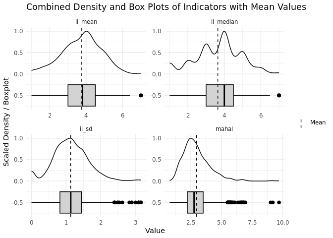
The density and box plots provide a quick visualization of central tendency and variability parameters for each calculated indicator. Box plots highlight key summary statistics like the median, quartiles, and potential outliers, while density plots complement this by showing the distribution shape and peaks. Together, they give us a full picture of how response patterns across the items of the scales are distributed in our sample.
The resp_distributions function provides two measures of central tendency: ii_mean (average response) and ii_median (central response) for each respondent.
From our output on the distribution of both parameters across all respondents of the 10-item scale of institutional trust (ranging from 1 to 7), we can conclude the following:
- The mean of
ii_meanis 3.76, and the median ofii_meanis 3.80. These parameters tell us that the average respondent selects a mean response with the value 3.8 across all items of the institutional trust scale. Looking at the median ofii_mean, we see that 50% of our respondents select a mean response up to the value of 4 across all items. The plot additionally indicates a nearly normal distribution ofii_meanwith a slight skew towards lower values. - The
ii_medianhas a mean value of 3.65 and a median value of 4.0. These parameters indicate that on average 50% of the given answers across the items of the institutional trust scale lie below the value of 3.7 and that half of the respondents give a value up to 4 for 50% of their responses across the items of the institutional trust scale. - Box plots for both indicators further undermine these parameters by showing that half of the respondents have scores between the values 3.0 and 4.5. Respondents selecting the upper endpoint of the scale (i.e., “7”) are outliers, while selecting the lower scale endpoint lies within a normal range.
In summary, the distributions of central tendency parameters show a concentration of responses around the value 4 which could indicate respondents’ tendency to select the mid-point or answers close to the mid-point of the scale avoiding giving extreme responses. Outliers among others are respondents who show a mean or median response across all items at the upper end of the response scale (“Entirely trust”). These respondents might need further checks to exclude the possibility of data quality issues.
resp_distributions also provides two measures of variability: ii_sd (individual response variability) and mahal (deviation from overall response patterns). From the output on the distribution across all respondent, we can see the following:
The mean
ii_sdis 1.13, meaning, on average, respondents’ answers across the items of the scale vary by about 1 point from their average response across all items.The third quartile of
ii_sdis 1.45, meaning 75% of respondents have moderate variability in their responses, with some showing higher fluctuations around their personal mean response across items. According to the box plot, those respondents with a variability exceeding the value of 2.5 are outliers among the other respondents.Mahalanobis distance (
mahal) does not have a straightforward interpretation likeii_sd. However, respondents withmahalscores slightly above 5 exhibit highly dissimilar response patterns compared to the overall average response pattern across items. These outliers could indicate potential data quality concerns and it might be worthwhile to examine these respondents in more detail.
In summary, most respondents show moderate variability indicating consistent responding, which again might point towards a tendency to select non-extreme answers close to the mid-point of the scale. A few respondents show a somewhat high variability in their responses which could call for additional checks to assess whether their responses reflect poor response behavior. Mahalanobis distance can further hint at respondents whose patterns deviate substantially from the average response pattern across all respondents which might be a sign of poor response behavior.
Straightlining or non-differentiation
From the standard deviation across items we can additionally infer whether respondents show straightlining response behavior across the multiple items of each scale. Straightlining or non-differentiation describes the response pattern of selecting the identical answer to a series of questions or items of a scale. It can indicate whether a respondent properly processed the respective question(s) or used shortcuts to reduce cognitive burden which in turn produces poor quality answers that do not represent a respondents’ true values. To get a measure for straightlining response behavior, we generate a new indicator based on a respondents’ standard deviation across the several items:
# Generating straightlining indicator for institutional trust scale
trust_distribution$non_diff <- NA
trust_distribution$non_diff[trust_distribution$ii_sd == 0] <- 1
trust_distribution$non_diff[trust_distribution$ii_sd != 0] <- 0

# Calculate proportion of respondents who show straightlining response behavior
trust_straightline_df <- data.frame(
  Indicator = "Straightlining Respondents",
  Proportion = round(prop.table(table(trust_distribution$non_diff))[2], 4)
)

# Print the result as a table
kable(trust_straightline_df, col.names = c("Trust Scale", "Proportion"))| Trust Scale | Proportion |
|---|---|
| Straightlining Respondents | 0.0514 |
Note
Apart from a binary measure indicating the selection of the identical response option across items versus selecting at least two different response options across a set of items is only one of several possible operationalizations of straightlining or non-differentiation. For an overview of the different possible operationalizations used in research, see Kim et al. (2019).
The results show that about 5% of respondents show straightlining response behavior in the institutional trust scale, meaning that 5% of respondents selected the identical answer across the several items. This is a relatively low proportion of straightlining behavior across respondents and does not indicate general data quality issues. However, it is necessary to flag these respondents who show straightlining across the items of a scale for a further investigation of their response behavior. The code below creates a new variable in the dataset, flagging respondents who show straightlining across the items of the institutional trust scale as TRUE; otherwise, as FALSE.
# Flag respondents with zero variation in responses (ii_sd == 0)
trust_distribution$straightlining_flag <- trust_distribution$ii_sd == 0
Be careful! Whereas straightlining can indicate “careless” response behavior resulting in poor quality responses, we advise to always pay attention to the contents of the several items of a scale before drawing conclusions. For some multi-item scales, selecting identical answers across all the items can be plausible and reflect respondents’ true values. On the other hand, some scales comprise reversely coded items, meaning that selecting the identical answer for such items is contradictory regarding the surveyed attitude or behavior. In this case straightlining might be more likely implausible and might more likely represent poor quality responses. In this case, however, all items are identically polarized and cover trust in several official institutions. Showing the identical answer across all items might reflect genuine distrust or trust in institutions overall. To make sure that you are in fact identifying careless respondents, we advise to look at respondents’ response times for the question at hand. Identifying extremely low response times against this background is a common strategy to approach the question of whether respondents did not pay attention to the question or show genuine undifferentiated answers.
2. NEP Scale
Now let’s move on to inspecting the central tendency and variability parameters for the NEP scale:
# Summarize and print results over all respondents
NEP_table <- summary(NEP_distribution)
kable(NEP_table)| n_na | prop_na | ii_mean | ii_sd | ii_median | mahal | |
|---|---|---|---|---|---|---|
| Min. : 0.000 | Min. :0.0000 | Min. :1.000 | Min. :0.0000 | Min. :1.000 | Min. :1.517 | |
| 1st Qu.: 0.000 | 1st Qu.:0.0000 | 1st Qu.:2.467 | 1st Qu.:0.9155 | 1st Qu.:2.000 | 1st Qu.:2.914 | |
| Median : 0.000 | Median :0.0000 | Median :2.667 | Median :1.1212 | Median :2.000 | Median :3.540 | |
| Mean : 2.749 | Mean :0.1833 | Mean :2.639 | Mean :1.1516 | Mean :2.335 | Mean :3.710 | |
| 3rd Qu.: 0.000 | 3rd Qu.:0.0000 | 3rd Qu.:2.867 | 3rd Qu.:1.3870 | 3rd Qu.:3.000 | 3rd Qu.:4.334 | |
| Max. :15.000 | Max. :1.0000 | Max. :3.733 | Max. :2.0656 | Max. :5.000 | Max. :8.170 | |
| NA | NA | NA’s :285 | NA’s :285 | NA’s :285 | NA’s :285 |
# Reshape the data for density and box plots
NEP_distribution_long <- pivot_longer(NEP_distribution,
                                         cols = c("ii_mean", "ii_sd", "ii_median", "mahal"),
                                         names_to = "Indicator",
                                         values_to = "Value")

# Remove non-finite values
NEP_distribution_long <- NEP_distribution_long %>%
  filter(!is.na(Value) & is.finite(Value))

# Calculate mean for each Indicator
mean_values <- NEP_distribution_long %>%
  group_by(Indicator) %>%
  summarize(mean_value = mean(Value, na.rm = TRUE))

# Create combined boxplot and density plot with a dashed line for each mean
ggplot(NEP_distribution_long, aes(x = Value, y = after_stat(scaled))) +
  geom_density(aes(y = after_stat(scaled)), alpha = 0.5) +
  geom_boxplot(aes(y = -0.5), width = 0.5, outlier.size = 2, color = "black", fill = "lightgray") +
  geom_vline(data = mean_values, aes(xintercept = mean_value, color = "Mean"), linetype = "dashed") +
  scale_color_manual(values = c("Mean" = "black")) +
  facet_wrap(~ Indicator, scales = "free") +
  labs(title = "Combined Density and Box Plots of Indicators with Mean Values",
       x = "Value",
       y = "Scaled Density / Boxplot") +
  theme_minimal() +
  theme(legend.position = "right",
        legend.title = element_blank()) # Remove legend title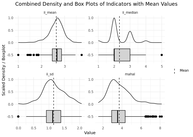
Again, the output shows the distribution of the central tendency parameters across all respondents. For the 15-item NEP scale (ranging from 1 to 5), our central tendency measures show the following:
- The mean of
ii_meanis 2.64, and the median ofii_meanis 2.67. According to these parameters, the average respondent shows a personal mean response of 2.6 across all items of the scale whereas half of the respondents give a mean response across all items up to the value of 2.7. The plots show an almost normal distribution centered around the mid-point of the scale. Respondents with mean responses at the lower end (agree) and upper end (disagree) of the scale are outliers among the other respondents in the sample. - The
ii_medianhas a mean value of 2.34 and a median value of 2.0. These parameters suggest that on average 50% of given answers to the items of the scale lie below the value of 2.3 and that for half of the respondents 50% of their answers to the items of the NEP scale lie below the value of 2. The plots further undermine this by showing a noticeable concentration of responses at the values 2 and 3. Respondents with a median response of “fully disagree” are outliers among the other respondents.
In summary, the distributions of the calculated central tendency indicators again show clustering of responses around the values 2 and 3 with 3 representing the scale mid-point. This clear concentration around the mid-points of the scale could again indicate respondents’ tendency to select scale mid-points rather than extreme answers. Respondents with mean extreme responses of both full agreement or full disagreement are outliers in the sample and might need additional checks to exclude data quality issues.
From the output of the distribution of variability measures across all respondents, we can conclude:
The mean
ii_sdis 1.15, which indicates that, on average, responses across all items vary by about 1 point from their individual mean response across items. While somewhat higher fluctuations up to 2 are within the normal range among the sample, no fluctuation at all (ii_sd= 0), meaning that respondents select the identical answer for every item is an outlier.The plot displaying the distribution of the Mahalanobis distance (
mahal) across all respondents shows that respondents with amahalscore near or above 6 are outliers in the sample with atypical responses, compared to the average responding pattern of the other respondents.
In summary, most respondents show some variability across the items of the scale, however, a few respondents show no variability at all meaning they provide identical answers across all items and are outliers compared to the rest of the sample. These respondents along with respondents who are extremely dissimilar from the average response pattern (indicated by the mahal indicator) should be further investigated as they could exhibit poor response behavior. We especially assume a data quality concern regarding respondents who show zero variability in responses, that is show straightlining.
Straightlining or non-differentiation
Unlike the institutional trust scale, the NEP scale comprises several reversely coded items (i.e., meaning that some of the items are positively formulated while others are negatively worded with respect to environmental attitudes). To better understand the difference, we have to look at the item contents again:
Question: To what extent do you agree or disagree with the following statements?
Response Scale: 1 = Fully agree; 2 = Agree; 3 = Neither nor; 4 = Don’t agree; 5 = Fully disagree
Items:
- We are approaching the limit of the number of people the earth can support (Pro-environmental)
- Humans have the right to modify the natural environment to suit their needs (Anti-environmental)
- When humans interfere with nature it often produces disastrous consequences (Pro-environmental)
- Human ingenuity will ensure that we do NOT make the earth unlivable (Anti-environmental)
- Humans are severely abusing the environment (Pro-environmental)
- There are enough resources on the planet - we just have to learn how to use them (Anti-environmental)
- Plants and animals have as much right as humans to exist (Pro-environmental)
- The balance of nature is strong enough to cope with the impacts of modern industrial nations (Anti-environmental)
- Despite our special abilities humans are still subject to the laws of nature (Pro-environmental)
- The so called ‘ecological crisis’ facing humankind has been greatly exaggerated (Anti-environmental)
- The earth is like a spaceship with very limited room and resources (Pro-environmental)
- Humans were meant to rule over the rest of nature (Anti-environmental)
- The balance of nature is very delicate and easily upset (Pro-environmental)
- Humans will eventually learn enough about how nature works to be able to control it (Anti-environmental)
- If things continue on their present course, we will soon experience a major ecological catastrophe (Pro-environmental)
8 of the items are “positively” worded, with a response of 1 indicating a pro-environmental attitude. In contrast, the remaining 7 items are “negatively” worded, where a response of 1 indicates an anti-environmental attitude. As a result, respondents showing straightlining (i.e., giving the identical response to all items) contradict attitudinal aspects of previous items, suggesting respondents indeed show careless responding. This is especially true if respondents select identical responses at the extremes of the scale. However, we have to again be careful with hasty conclusions: In the case of respondents straightlining across the mid-point of the scale, we cannot immediately rule out the possibility of genuine ambiguity and should perform further checks to examine the possibility of poor quality responses. Nevertheless, straightlining in the NEP scale might especially pose a threat for data quality and should be investigated:
# Generating straightlining indicator for institutional trust scale
NEP_distribution$non_diff <- NA
NEP_distribution$non_diff[NEP_distribution$ii_sd == 0] <- 1
NEP_distribution$non_diff[NEP_distribution$ii_sd != 0] <- 0

# Calculate proportion of respondents who show straightlining response behavior
NEP_straightline_df <- data.frame(
  Indicator = "Straightlining Respondents",
  Proportion = round(prop.table(table(NEP_distribution$non_diff))[2], 4)
)

# Print the result as a table
kable(NEP_straightline_df, col.names = c("NEP Scale", "Proportion"))| NEP Scale | Proportion |
|---|---|
| Straightlining Respondents | 0.0053 |
For the NEP scale, we can see that 0.5% of respondents show straightlining across the several items of the scale. Despite the low prevalence of straightlining in the data, respondents who straightlined in the NEP scale are highly likely to show poor quality responses and should be flagged for further analyses. Below, we again flag respondents who show straightlining across the items of the NEP scale with a new variable named straightlining_flag:
# Flag respondents with zero variation in responses (ii_sd == 0)
NEP_distribution$straightlining_flag <- NEP_distribution$ii_sd == 0
Be careful! As the NEP scale includes items with both positive and negative wordings, the response distribution indicators cannot be directly used for the description of the distribution of pro- or anti-environmental attitudes. To derive substantively meaningful conclusions from the indicators (e.g., average environmental attitudes among the respondents), it’s necessary to reverse-code either the positively or negatively worded items. This ensures that all items reflect the same directional attitude. For the recoding, you can use the following code chunk:
# Create a new data frame by copying the original NEP data
NEP_recoded <- NEP

# Reverse code the negatively worded items in the new data frame
NEP_recoded$bczd006a <- 6 - NEP_recoded$bczd006a  # Q2: Humans have the right to modify the natural environment
NEP_recoded$bczd008a <- 6 - NEP_recoded$bczd008a  # Q4: Human ingenuity
NEP_recoded$bczd010a <- 6 - NEP_recoded$bczd010a  # Q6: There are enough resources
NEP_recoded$bczd012a <- 6 - NEP_recoded$bczd012a  # Q8: The balance of nature is strong enough
NEP_recoded$bczd014a <- 6 - NEP_recoded$bczd014a  # Q10: Ecological crisis exaggerated
NEP_recoded$bczd016a <- 6 - NEP_recoded$bczd016a  # Q12: Humans were meant to rule over nature
NEP_recoded$bczd018a <- 6 - NEP_recoded$bczd018a  # Q14: Control nature
Calculating indicators of various response styles
After investigating the response distribution of both the institutional trust scale and the NEP scale, let’s now take a closer look on systematic response styles that can indicate poor quality responses in multi-item scales. For this, we use the resp_styles function of the resquin package, which calculates indicators for the following response styles:
Response Styles:
Mid-point response style (MRS): Tendency to choose the mid-point of a response scale
Acquiescence (ARS): Tendency to agree with statements
Extreme Response Style (ERS): Tendency to select the endpoints of a response scale
To use resp_styles, we first need to specify the range of the response scale of the underlying multi-item scale or matrix question. Only with information on the range, and therefore on the existence of a mid-point and the endpoints of the response scale, resp_styles can calculate indicators for the different response styles. Similar to resp_distributions, we can additionally specify the proportion of valid responses respondents should have on the multi-item scale (min_valid_responses) to calculate response style indicators. To enable the calculation of all response style indicators per respondent, we only include those respondents who show no NAs across items. We can further determine whether we want resp_styles to simply return the counts of each response style across items or if it should return the proportion of a specific response behavior out of all the items a respondent has answered. Although the proportion of a certain response behavior is generally more informative than the mere count, we specify the option normalize = FALSE for our analysis in this tutorial.
# Calculating response style indicators for institutional trust
trust_respstyles <- resp_styles(trust, 1, 7, min_valid_responses = 1, normalize = FALSE)

# Print results of the first 10 respondents
kable(trust_respstyles[1:10,])| MRS | ARS | DRS | ERS | NERS |
|---|---|---|---|---|
| 1 | 2 | 7 | 0 | 10 |
| NA | NA | NA | NA | NA |
| 3 | 5 | 2 | 0 | 10 |
| 1 | 2 | 7 | 6 | 4 |
| 2 | 0 | 8 | 0 | 10 |
| 10 | 0 | 0 | 0 | 10 |
| 2 | 7 | 1 | 3 | 7 |
| 1 | 4 | 5 | 0 | 10 |
| 0 | 0 | 10 | 3 | 7 |
| 2 | 7 | 1 | 2 | 8 |
# Calculating response style indicators for environmental attitudes
NEP_respstyles <- resp_styles(NEP, 1, 5, min_valid_responses = 1, normalize = FALSE)

# Print results of the first 10 respondents
kable(NEP_respstyles[1:10,])| MRS | ARS | DRS | ERS | NERS |
|---|---|---|---|---|
| 1 | 4 | 10 | 3 | 12 |
| 0 | 7 | 8 | 4 | 11 |
| 0 | 8 | 7 | 0 | 15 |
| 5 | 4 | 6 | 0 | 15 |
| 1 | 6 | 8 | 4 | 11 |
| NA | NA | NA | NA | NA |
| 0 | 6 | 9 | 5 | 10 |
| 3 | 4 | 8 | 8 | 7 |
| 2 | 4 | 9 | 7 | 8 |
| 2 | 5 | 8 | 10 | 5 |
As with resp_distributions, resp_styles returns a data frame containing the several response style indicators per respondent (displayed as separate rows of the data frame). Again, let’s first inspect the calculated indicators for the first 10 respondents in our data frame: Similar to resp_distributions we see that for 1 out of the first 10 respondents of the institutional trust scale and for 1 out of the first 10 respondents of the NEP scale, no indicators were calculated due to our specification of min_valid_responses, which only included respondents without NA across items into the analysis.
Indicators of response styles
To make statements about the occurrence of the specific response styles in the institutional trust and NEP scale across all respondents, we have to again calculate and visualize summary statistics for each indicator in the data frame produced by resp_styles.
1. Institutional Trust Scale
Let’s again begin with the institutional trust scale.
# Summarize and print results over all respondents
trust_respstyles_table <- summary(trust_respstyles)
kable(trust_respstyles_table)| MRS | ARS | DRS | ERS | NERS | |
|---|---|---|---|---|---|
| Min. : 0.000 | Min. : 0.000 | Min. : 0.000 | Min. : 0.000 | Min. : 0.000 | |
| 1st Qu.: 1.000 | 1st Qu.: 1.000 | 1st Qu.: 1.000 | 1st Qu.: 0.000 | 1st Qu.: 8.000 | |
| Median : 2.000 | Median : 3.000 | Median : 4.000 | Median : 0.000 | Median :10.000 | |
| Mean : 2.443 | Mean : 3.254 | Mean : 4.302 | Mean : 1.392 | Mean : 8.608 | |
| 3rd Qu.: 4.000 | 3rd Qu.: 5.000 | 3rd Qu.: 7.000 | 3rd Qu.: 2.000 | 3rd Qu.:10.000 | |
| Max. :10.000 | Max. :10.000 | Max. :10.000 | Max. :10.000 | Max. :10.000 | |
| NA’s :250 | NA’s :250 | NA’s :250 | NA’s :250 | NA’s :250 |
# Reshape the data for density and box plots
trust__respstyles_long <- pivot_longer(trust_respstyles,
                                         cols = c("MRS", "ARS", "ERS"),
                                         names_to = "Indicator",
                                         values_to = "Value")

# Remove NAs (for those we have no calculated indicators)
trust__respstyles_long <- trust__respstyles_long %>%
  filter(!is.na(Value))

# Calculate mean for each Indicator
mean_values <- trust__respstyles_long %>%
  group_by(Indicator) %>%
  summarize(mean_value = mean(Value, na.rm = TRUE))

# Create combined boxplot and density plot with a dashed line for each mean
ggplot(trust__respstyles_long, aes(x = Value, y = after_stat(scaled))) +
  geom_density(aes(y = after_stat(scaled)), alpha = 0.5) +
  geom_boxplot(aes(y = -0.5), width = 0.5, outlier.size = 2, color = "black", fill = "lightgray") +
  geom_vline(data = mean_values, aes(xintercept = mean_value, color = "Mean"), linetype = "dashed") +

  scale_color_manual(values = c("Mean" = "black")) +
  facet_wrap(~ Indicator, scales = "free") +
  labs(title = "Combined Density and Box Plots of Indicators with Mean Values",
       x = "Value",
       y = "Scaled Density / Boxplot") +
  theme_minimal() +
  theme(legend.position = "right",
        legend.title = element_blank())  # Remove legend title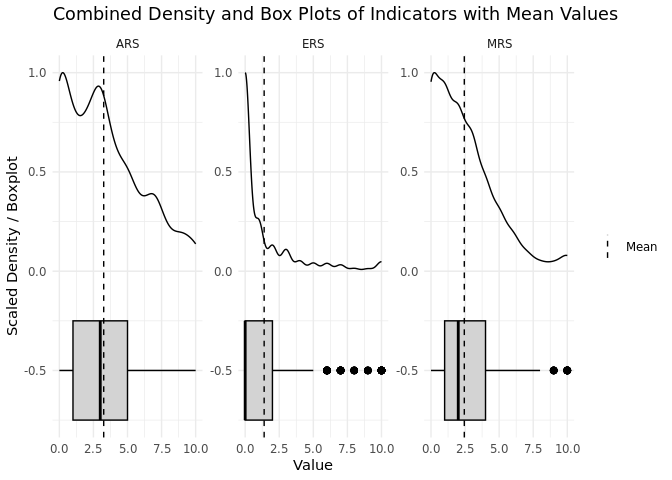
Looking at the response style indicators across all respondents of the institutional trust scale, we see the following patterns:
MRS: On average, respondents in our sample tend to select the midpoint of the scale (response of the value 4) for about two out of ten items. The boxplot shows that selecting anywhere between 0 to 8 midpoint responses across the items of the scale lies within the normal range among the sample. However, respondents who select the scale mid-point for 9 or 10 items are outliers, reflecting an usual high amount of given mid-point answers in the sample.
ARS: On average, respondents “agree” with about three out of ten items. The ARS indicator defines agreement as selecting response options above the scale mid-point, that is every response that indicates some level of trust toward a specific institutions or in other words, “agrees” with the trustworthiness of that institution. While 75% of respondents do not agree with more than five out of the ten items, agreement up to every item of the scale falls within the typical distribution range of the sample and does so far not raise any concerns for the response quality of the institutional trust scale.
ERS: On average, respondents select extreme responses (i.e., the lower and upper endpoint of the scale) for only one out of ten items. Moreover, the majority of respondents does not provide more than two extreme responses across the items of the scale. Respondents providing more than five extreme responses are outliers in the sample, indicating a potential bias of those responses.
In summary, the investigated response style indicators reveal that the majority of respondents does not show an excessive use of the mid-point as well as the endpoints of the institutional trust scale. Respondents who (almost) consistently select middle responses (which could also indicate straightlining behavior) and respondents with more than five extreme responses across items are outliers. These respondents should be further checked for anomalies in their response behavior (e.g., their response times) to exclude data quality concerns.
Be careful! When interpreting the indicator of acquiescence response style (ARS), be aware that strictly speaking you can only meaningfully interpret the indicator for actual agreement/disagreement - scales. For the purpose of this tutorial, we calculated and interpreted it for the trust scale ranging from complete distrust to complete trust to show how to extract some information about potential data quality issues from it. However, for scientific publications or data quality reports, we recommend to not use the ARS-indicator for scales other than agreement/disagreement - scales. Be also aware that the calculation of the ARS indicator assumes that the response scale is positively polarized, i.e., higher values of the response scale reflect higher levels of agreement with certain statements or issues.
Package-specific feature Apart from MRS, ARS, and ERS, the resquin-package additionally calculates an indicator for disacquiescence response style (DRS), i.e., the tendency to disagree with statements, and an indicator for non-extreme response style (NERS), i.e., the tendency to select non- extreme answers across a set of items. When interpreting the indicators for these response styles, keep in mind that the DRS-indicator is the direct opposite of the ARS-indicator and the NERS-indicator is the direct inverse of the ERS-indicator. Especially, for NERS and ERS it might be pointless to meaningfully interpret both indicators at the same time.
2. NEP Scale
Be careful! Remember that ARS reflects the tendency to agree with statements. The calculation of ARS in the resquin package (i.e., sum of answers above the scale mid-point across all items of the scale) assumes a positively polarized scale, where higher values indicate stronger agreement. However, the NEP scale is negatively polarized, with lower values indicating agreement (1 = fully agree). To compute ARS accurately, we need to reverse-code all the items so that 5 indicates agreement and 1 indicates disagreement. After this transformation, we should then recalculate the response style indicators on the reverse-coded data to be able to interpret them accordingly.
# Define the columns to reverse-code
NEP_columns <- colnames(NEP)  # Replace with specific columns if needed

# Create a reversed version of NEP data and perform reverse-coding to positively polarize the scale
NEP_positively_polarized <- NEP
NEP_positively_polarized[NEP_columns] <- 6 - NEP[NEP_columns]

# Calculate response style indicators on the positively polarized NEP data
NEP_positively_polarized_respstyles <- resp_styles(NEP_positively_polarized, 1, 5,min_valid_responses = 1,normalize = FALSE)
Let’s now inspect response style indicators for the (recoded) positively polarized NEP scale:
# Summarize and print results over all respondents
NEP_positively_polarized_respstyles_table <- summary(NEP_positively_polarized_respstyles)
kable(NEP_positively_polarized_respstyles_table, format = output_format)| MRS | ARS | DRS | ERS | NERS | |
|---|---|---|---|---|---|
| Min. : 0.000 | Min. : 0.000 | Min. : 0.000 | Min. : 0.000 | Min. : 0.00 | |
| 1st Qu.: 1.000 | 1st Qu.: 7.000 | 1st Qu.: 3.000 | 1st Qu.: 1.000 | 1st Qu.: 9.00 | |
| Median : 2.000 | Median : 8.000 | Median : 5.000 | Median : 3.000 | Median :12.00 | |
| Mean : 2.327 | Mean : 8.211 | Mean : 4.462 | Mean : 3.639 | Mean :11.36 | |
| 3rd Qu.: 3.000 | 3rd Qu.: 9.000 | 3rd Qu.: 6.000 | 3rd Qu.: 6.000 | 3rd Qu.:14.00 | |
| Max. :14.000 | Max. :15.000 | Max. :11.000 | Max. :15.000 | Max. :15.00 | |
| NA’s :285 | NA’s :285 | NA’s :285 | NA’s :285 | NA’s :285 |
# Reshape the data for density and box plots
NEP_positively_polarized_respstyles_long <- pivot_longer(NEP_positively_polarized_respstyles,
                                         cols = c("MRS", "ARS", "ERS"),
                                         names_to = "Indicator",
                                         values_to = "Value")

# Remove NAs (for those we have no calculated indicators)
NEP_positively_polarized_respstyles_long <- NEP_positively_polarized_respstyles_long %>%
  filter(!is.na(Value))

# Calculate mean for each Indicator
mean_values <- NEP_positively_polarized_respstyles_long %>%
  group_by(Indicator) %>%
  summarize(mean_value = mean(Value, na.rm = TRUE))

# Create combined boxplot and density plot with a dashed line for each mean
ggplot(NEP_positively_polarized_respstyles_long, aes(x = Value, y = after_stat(scaled))) +
  geom_density(aes(y = after_stat(scaled)), alpha = 0.5) +
  geom_boxplot(aes(y = -0.5), width = 0.5, outlier.size = 2, color = "black", fill = "lightgray") +
  geom_vline(data = mean_values, aes(xintercept = mean_value, color = "Mean"), linetype = "dashed") +

  scale_color_manual(values = c("Mean" = "black")) +
  facet_wrap(~ Indicator, scales = "free") +
  labs(title = "Combined Density and Box Plots of Indicators with Mean Values",
       x = "Value",
       y = "Scaled Density / Boxplot") +
  theme_minimal() +
  theme(legend.position = "right",
        legend.title = element_blank())  # Remove legend title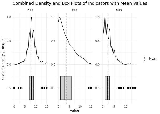
The distribution of response style indicators across all respondents of the NEP-scale, reveals the following patterns:
MRS: Respondents on average select the middle response category for two out of the 15 items of the NEP scale. Respondents with more than six mid-point responses are outliers in the sample while respondents maximally selected 14 mid-point responses for the 15 items. Similarly to the institutional trust scale, this distribution pattern suggest that mid-point responding is not a dominant response style for the NEP scale among our sample. Therefore, outliers should be carefully checked regarding their response behavior to exclude data quality issues.
ARS: On average, respondents show a reasonable amount of agreeing responses by agreeing with about eight out of 15 items. Against the background of reversely coded items (i.e.,eight items are formulated pro-environmental and 7 items are formulated anti-environmental) the amount of average agreeing responses across the items indicates that responses are not generally affected by acquiescence bias and of poor quality as on average respondents do not report conflicting attitudes. However, some respondents show an unreasonable amount of agreeing responses across items as we can see from the distribution plot. In addition, the outcome shows that on maximum respondents agree with all of the items of the scale irrespective of their opposite wording. Although, according to the distribution plots, respondents are only outliers in the sample if they agreed to more than 12 items, we recommend flagging every respondent with more than eight agreeing responses due to the design of the scale. These respondents should be closely checked regarding their response behavior, and additional proxies, such as their response times, should be investigated to gain further insights into the quality of their responses.
ERS: On average, respondents select the extreme end-points of the scale to about three to four out of 15 items. Respondents with more than 13 extreme responses across the items of the scale are considered outliers in the sample. Overall, the distribution suggests that respondents indeed avoid extreme answers and stick to more moderate positions. Consequently, those with a high amount of given extreme responses and respondents who provided endpoint responses to all of the 15 items of the scale should be carefully investigated regarding any data quality concerns.
In summary, the distribution of response style indicators for the NEP-scale suggests that the measure is generally not affected by any of the observed response styles (i.e., MRS, ARS, and ERS). However, some outliers give cause for data quality concerns and should be flagged for further investigation. Especially, our findings regarding agreement bias show concerning response patterns regarding the reverse wording of items in the scale. Respondents with more agreeing responses than positively or negatively formulated items should be flagged and closely inspected regarding the quality of their responses. This in particular true for those respondents who straightlined across the items of the scale.
Good to know Although resquin and resp_styles is typically designed for multi-item scales or matrix questions that share the same question introduction and response scale, it is also possible to evaluate “stand-alone” survey questions (e.g., attitudes toward governmental spending, attitudes toward social policies) from a broader topic (e.g., political attitudes) together. If you want to do so, it is crucial to only investigate those “stand-alone” questions together which have the same number of response options. Also, you want to make sure that the questions are not separated from each other in the questionnaire but are in a consecutive order. As long as the several questions are sequential and share the same response scale, it is possible to calculate meaningful indicators of response styles.
Conclusion and recommendations
Institutional Trust Scale Overall, responses of the institutional trust scale are not affected by any major response bias. However, we do find unusual response patterns regarding straightlining responses and outliers in the sample who showed an unusual extent of mid-point and extreme responding. These respondents should definitely be flagged and ideally, their response behavior should be investigated in greater detail.
NEP Scale Similarly, responses of the NEP scale are not generallly affected by any of the investigated response biases, although again, outliers give reason for data quality concerns. Additionally, we find straightlining response behavior with on overall, a low prevalence of only 0.5% of straightlining responses. However, these respondents most likely present a data quality concern due to the reversely coded nature of the scale. Similarly, some response patterns regarding ARS are especially concerning since they suggest data quality threats. Again, due to the reversely coded items of the scale, response patterns with more than eight or seven agreeing responses across items suggests poor data quality with responses detached from true values. Respondents with suspicious response behaviors should be flagged and ideally further checked.
Straightlining: Straightlining response behavior is generally seen as a sign of low engagement and of respondents providing only minimal effort in the response generation process, which can potentially compromise data quality. However, we advise against interpreting straightlining behavior blindly as a data quality issue. Dependent on the underlying response scale and the construct to be measured, straightlining can sometimes reflect valid and genuine responses. One useful criterion to assess whether straightlining can be valid or reflects poor quality responses is to determine whether the underlying scale contains reversely coded items. In our example, we cannot fully exclude the possibility that straightlining response behavior in the institutional trust scale indicates genuine trust or distrust across all listed institutions or a respondents’ genuine indifference, especially in the case of the absence of a “don’t know” - response option. For the NEP-scale on the other hand, straightlined responses across item contradict each other as half of the items measure pro-environmental and the other half anti-environmental attitudes. Therefore, we recommend to always pay attention to the construct measured and how the scale measures it to assess whether all straightlining respondents are a severe threat to data quality.
Acquiescence response style: Acquiescence bias is again considered a sign of respondents’ low engagement with a question that results in poor quality responses. In multi-item scales, acquiescence bias is somewhat tricky to determine. Similarly to straightlining response behavior, high shares of agreeing responses across items does not necessarily reflect response bias. Scales measuring widely accepted values for instance, can show high agreement among respondents without reflecting an acquiescence bias that indicates poor response quality. However, again the underlying scale can provide information on the severeness of an acquiescence response pattern across items. In the case of the NEP-scale with conflicting statements/items, a high share of agreeing responses give reason for concern and most likely represent biased responses. In general, we advise to take acquiescence response styles seriously and to assess their implications for the responses of a multi-item scale based on the content and formulation of items.
Outliers: We recommend to deal with outliers in the sample regarding both response distribution and response style indicators similarly to dealing with any outlier in a response distribution. First, you should attempt to understand the outlying observations and closely inspect the response behavior of these respondents. In any case, we advise against dropping these observations from the sample and instead, to flag these respondents for your further analyses.
Recommendation: Knowing how to assess and interpret indicators of response distribution and response styles regarding response quality, you probably wonder how to move on from there?
Ideally, we recommend to conduct further analyses on respondents with suspicious response patterns. A typical proxy to understand the response generation process underlying a response pattern and to understand whether responses represent a data quality issue are response times. If respondents show extremely short response times for a question, you can assume that respondents provided no to minimal effort to process the question which consequently resulted in poor quality responses. A common threshold to assess whether response times are too short to process a question is introduced by Zhang and Conrad (2014). Further measures to approach the question whether respondents’ answers reflect low engagement with a question and therefore, poor quality responses are respondent motivation or respondent cognitive ability. These are both factors discussed to influence the occurrence and magnitude of satisficing, an umbrella term for different response strategies that can be used as shortcuts to reduce cognitive burden and can therefore, reflect careless responding (Krosnick 1991).
For your further analyses, we recommend in any case to not simply drop respondents with suspicious response patterns. Instead, we advise to always flag them and run sensitivity analyses both including and excluding the respective respondents to gain insights on whether their responses affect your overall findings.
References
Dunlap, Riley E., Kent D. Van Liere, Angela G. Mertig, and Robert Emmet Jones. 2002. “New Trends in Measuring Environmental Attitudes: Measuring Endorsement of the New Ecological Paradigm: A Revised NEP Scale.” Journal of Social Issues 56 (3): 425–42. https://doi.org/10.1111/0022-4537.00176.
GESIS Panel, Team. 2017. “GESIS Panel - Campus File.” GESIS Data Archive, Cologne. ZA5666 Data file Version 1.0.0. https://doi.org/10.4232/1.12749.
Kim, Yujin, Jennifer Dykema, John Stevenson, Peter Black, and Daniel P. Moberg. 2019. “Straightlining: Overview of Measurement, Comparison of Indicators, and Effects in Mail–Web Mixed-Mode Surveys.” Social Science Computer Review 37 (2): 214–33. https://doi.org/10.1177/0894439317752406.
Krosnick, J. A. 1991. “Response Strategies for Coping with the Cognitive Demands of Attitude Measures in Surveys.” Applied Cognitive Psychology 5 (3): 213–36. https://doi.org/10.1002/acp.2350050305.
Roth, Matthias, Nivedita Bhaktha, Matthias Bluemke, Thomas Knopf, Fabienne Krämer, Clemens Lechner, and Çağla Yildiz. 2024. “Resquin: Response Quality Indicators for Survey Research.” R package version 0.0.2. https://doi.org/10.32614/CRAN.package.resquin.
Zhang, C., and F. Conrad. 2014. “Speeding in Web Surveys: The Tendency to Answer Very Fast and Its Association with Straightlining.” Survey Research Methods 8: 127–35. https://doi.org/10.18148/srm/2014.v8i2.5453.
Reuse
Citation
BibTeX citation:
@misc{kraemer2024,
  author = {Kraemer, Fabienne and Eser, Arjin and Yıldız, Çağla and
    Roth, Matthias},
  publisher = {GESIS – Leibniz Institute for the Social Sciences},
  title = {Assessing {Response} {Quality} and {Careless} {Responding} in
    {Multi-Item} {Scales}},
  date = {2024-11-04},
  urldate = {2025-05-19},
  url = {https://github.com/kraemefe/resquin-tool-application},
  langid = {en}
}
For attribution, please cite this work as:
Kraemer, Fabienne, Arjin Eser, Çağla Yıldız, and Matthias Roth. 2024.
“Assessing Response Quality and Careless Responding in Multi-Item
Scales.” KODAQS Toolbox. GESIS – Leibniz Institute for
the Social Sciences. https://github.com/kraemefe/resquin-tool-application.